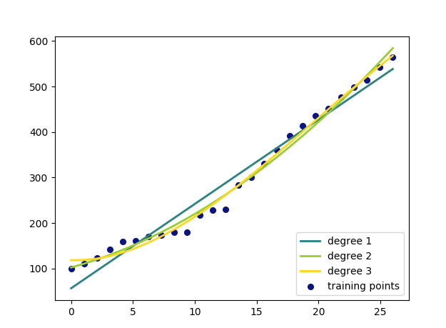
Polynomial regression is a process of finding a polynomial function that takes the form f( x ) = c0 + c1 x + c2 x2 ⋯ cn xn where n is the degree of the polynomial and c is a set of coefficients. Through polynomial regression we try to find an nth degree polynomial function which is the closest approximation of our data points. Below is a sample random dataset which has been regressed upto 3 degree and plotted on a graph. The blue dots represent our data set and the lines represent our polynomial functions of different degrees. The higher the degree, closer is the approximation but higher doesn’t always mean right which we will discuss in later articles.
y_train=[[100],[110],[124],[142],[159],[161],[170],[173],[179],[180],[217],[228],[230],[284],[300],[330],[360],[392],[414],[435],[451],[476],[499],[515],[543],[564]]
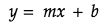
To understand the math behind the above analysis lets start by constructing a line function that passes through two points: (1, 1) and (6, 9). The general formula of the equation of line:
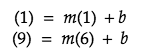
Our job here is to find the two unknowns m and b in the above line equation. By putting our sample points in the above line equation, we get:
we can solve for m and b using substitution method:
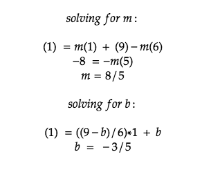
Now substituting m and b in our line equation, we get the below formula:

The above algebraic method works best for small number and one degree polynomials but for higher degree polynomials we will be using matrices and linear algebra. But before we dive into the math of higher degree functions lets work out the same equation we derived from our previous example using matrices.
Our data points in a matrix will look like:
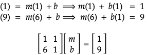
Solving it using linear algebra:

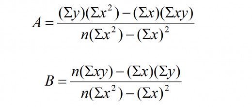
As you can see, we get the same equation of line using matrix and linear algebra. The above method works great when we have 2 points because we know we can draw a straight line passing through them but we cannot assure the same when we have more than 2 data points. In my article on linear regression I used the below formula to find the coefficients of linear equation y = Bx + A.
How we derive the above equation will give us the general formula for a polynomial function of any degree.
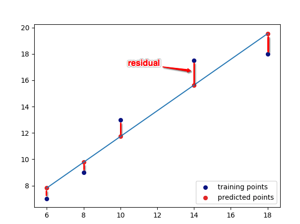
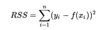
In any regression analysis we try to find an equation of line which is a close approximation of the actual training data points. We use a method called the “Sum of Least squares” to derive our equation. Basically what do is find all possible line equations for a given set of data points and select the one which has the least squared sum of errors or residuals – Residuals or errors being the difference between the predicted value and the actual value.
Least squares has been beautifully explained in the below video:
Sum of least squares as we saw in our previous article is given by :
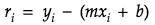
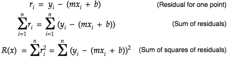
So for any point on a graph the residual is given by the general form:
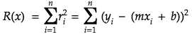
and the sum of squares of residuals become:
Now if we have to find a regression function then we will have to find an equation which gives the least sum of errors. We will be using partial derivatives to find the minima of our sum of least squares function:
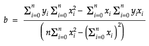
Taking the derivatives with respect to m and b we get:
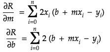
Now equating the partial derivatives to 0 to find the minimum value of m and b we get:
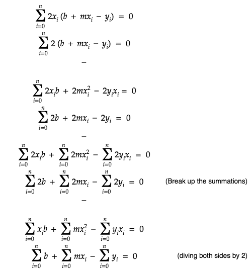
Moving the constants out and also moving y to the right side
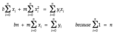
The second equation above can be represented with b on the left side:

substituting b in equation 1 we can find the formula to calculate m
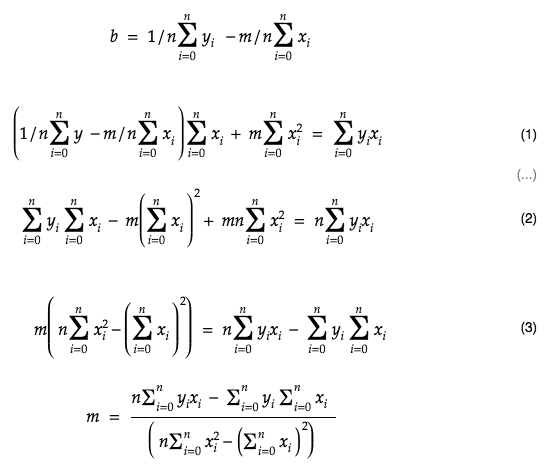
in the similar fashion we can also derive the formula for b
We derived the above formulas using algebra, we could have done it using matrices as well. Our initial two equations given by:
when represented in a matrix form looks like:
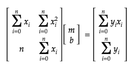
Evaluating the above we would get the same formula we found using algebra.
Lets see if we can extend the same method to derive a generic formula for higher degree polynomials. To start, lets use a quadratic equation represented by :
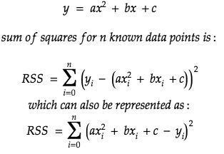
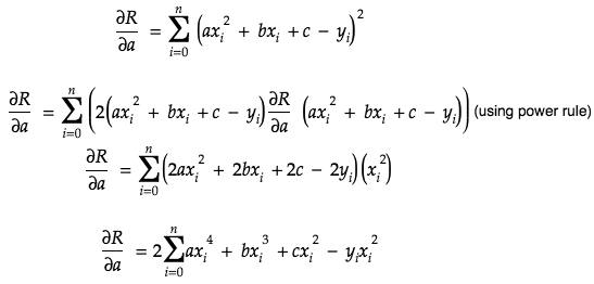
As you can see we have 3 coefficients a, b and c in the equation. Partials derivate of a is given by:
partial derivative of b:
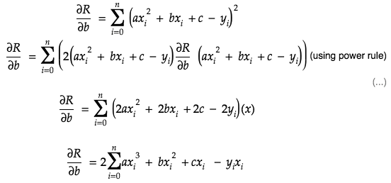
partial derivative of c:

Now to find the minima, we will set the partial derivatives to 0.

We can represent the above equations in matrix form:
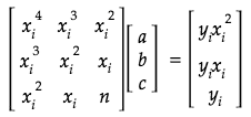
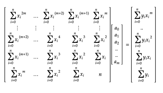
So, if m is the degree of the polynomial, and n is the number of known data points, we get a generalized matrix: