Previously we built a simple linear regression model using a single explanatory variable to predict the price of pizza from its diameter. But in the real world the price of pizza cannot be entirely derived from the diameter of its base alone. It also depends on the toppings, which means there are a many more independent variables to be used in the prediction equation. A regression using multiple explanatory variables is called multiple linear regression. A simple linear regression uses a single explanatory variable with a single coefficient whereas a multiple linear regression uses a coefficient for each explanatory variables but a single dependant variable.
The equation of multiple linear regression looks like:
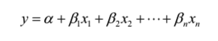
where x1,x2……xn represent our explanatory variables and y is our dependant variable. Mathematics of multiple linear regression involves complex matrix operations, a more detailed explanation of which I will keep for another post.
In this post we will focus on building a multiple linear regression modal using the Framingham Heart Study data which is a long-term, ongoing cardiovascular cohort study on residents of the town of Framingham, Massachusetts. The study began in 1948 with 5,209 adult subjects from Framingham, and is now on its third generation of participants. Much of the now-common knowledge concerning heart disease, such as the effects of diet, exercise, and common medications such as aspirin, is based on this study. One of the important observations from Framingham heart study was the strong correlation between BMI and blood pressure. People with higher BMI are at a higher risk of cardiovascular disease. Blood Pressure is also associated with rising age. Lets see if can derive these observations using our regression modal.
First, lets download the Framingham data from here. This dataset has a long list of columns from which we will be picking SYSBP, BMI, AGE, SEX and BPMEDS to build our modal.
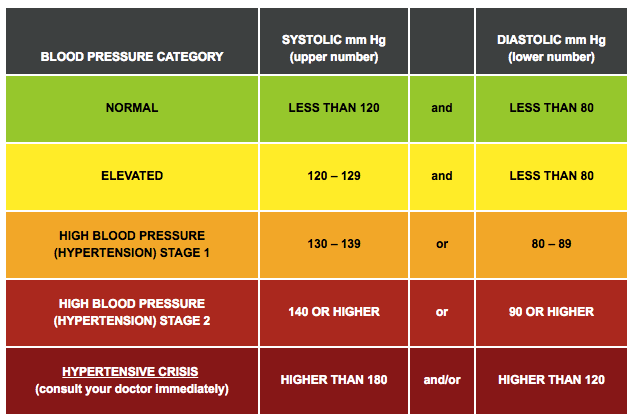
SYSBP – Systolic blood pressure is what we are trying to predict so it becomes our dependant variable Y. The below table shows the different categories of BP with their standard values.
BMI, AGE, SEX and BPMEDS (an indicator for antihypertensive medication use), all four variables will be our explanatory variable X. The standard values of BMI are as below:
- Underweight: Your BMI is less than 18.5
- Healthy weight: Your BMI is 18.5 to 24.9
- Overweight: Your BMI is 25 to 29.9
- Obese: Your BMI is 30 or higher
1. Importing the data – We would be using pandas library for importing our data into a dataframe. A short introduction to pandas library can be found here.
import pandas as pd

# Importing the dataset
dataset = pd.read_csv('fram1.csv')
#ignoring a few null values from the dataset.
dataset = dataset[~dataset['BMI'].isnull()]
X = dataset.iloc[:, [0,8,3,6]].values #select SEX,BMI,AGE,CURSMOKE #,3,6
y = dataset.iloc[:, 4].values #select SYSBP
Upon trying to build the modal I found that few rows have the BMI empty, so I modified the program to remove null rows as you can see above.
2. Encoding the categorical data – The values in the field of SEX indicating male and female in the dataset is 1 and 2. We need to encode this using a label encoder which will give use 0 and 1 for Male and Female.
# Encoding categorical data
from sklearn.preprocessing import LabelEncoder

labelencoder = LabelEncoder()
X[:, 0] = labelencoder.fit_transform(X[:, 0])
3. Splitting the dataset into training and test set – This is an important aspect to model building which helps us in assessing our model’s predictive capabilities. The evaluation of which is done using the R-squared method. R-squared measures how well the observed values of the response variables are predicted by the model. In python we can simply use the score method to calculate the R-square. An r-squared score of 1 indicates that the response variable can be predicted without any error using the model. An r-squared score of one half indicates that half of the variance in the response variable can be predicted using the model.
# Splitting the dataset into the Training set and Test set
from sklearn.model_selection import train_test_split
X_train, X_test, y_train, y_test = train_test_split(X, y, test_size = 0.2, random_state = 0)
4. Fitting the Multiple regression to training set
# Fitting Multiple Linear Regression to the Training set
from sklearn.linear_model import LinearRegression
regressor = LinearRegression()
regressor.fit(X_train, y_train)

# Predicting the Test set results
y_pred = regressor.predict(X)

print 'R-squared: %.2f' % regressor.score(X_test, y_test)
print regressor.coef_
Outputs:
- R-squared: 0.26
- Regression Coef: 2.51226344 , 1.55951204, 0.92496226, -0.16286499
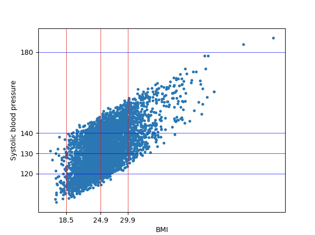
5. Plotting the output on a scatter chart.
fig, ax = plt.subplots()
ax.set_xticks([18.5, 24.9, 29.9], minor=False) #important values of BMI
ax.set_yticks([120, 130, 140, 180], minor=False) #important values of SysBP
ax.xaxis.grid(True, which='major',linewidth='0.5', color='red')
ax.yaxis.grid(True, which='major',linewidth='0.5', color='blue')

plt.scatter(X[:,1], y_pred, marker='.')
plt.ylabel("Systolic blood pressure")
plt.xlabel("BMI")
plt.show()
In the above plot we added appropriate grid lines to represent the various categories of BMI and SYS BP.
The entire program is as below:
# Multiple Linear Regression
# Importing the libraries
import numpy as np
import matplotlib.pyplot as plt
import pandas as pd
# Importing the dataset
dataset = pd.read_csv('fram1.csv')
dataset = dataset[~dataset['BMI'].isnull()] #ignoring a few null values from the dataset.
X = dataset.iloc[:, [0,8,3,6]].values #select SEX,BMI,AGE,CURSMOKE #,3,6
y = dataset.iloc[:, 4].values #select SYSBP
# Encoding categorical data
from sklearn.preprocessing import LabelEncoder, OneHotEncoder
labelencoder = LabelEncoder()
X[:, 0] = labelencoder.fit_transform(X[:, 0])
# Splitting the dataset into the Training set and Test set
from sklearn.model_selection import train_test_split
X_train, X_test, y_train, y_test = train_test_split(X, y, test_size = 0.2, random_state = 0)
# Fitting Multiple Linear Regression to the Training set
from sklearn.linear_model import LinearRegression
regressor = LinearRegression()
regressor.fit(X_train, y_train)
# Predicting the Test set results
y_pred = regressor.predict(X)
print 'R-squared: %.2f' % regressor.score(X_test, y_test)
print regressor.coef_
fig, ax = plt.subplots()
ax.set_yticks([18.5, 24.9, 29.9], minor=False) #important values of BMI
ax.set_xticks([120, 130, 140, 180], minor=False) #important values of SysBP
ax.yaxis.grid(True, which='major',linewidth='0.5', color='red')
ax.xaxis.grid(True, which='major',linewidth='0.5', color='blue')
plt.scatter(y_pred, X[:,1], marker='.')
plt.xlabel("Systolic blood pressure")
plt.ylabel("BMI")
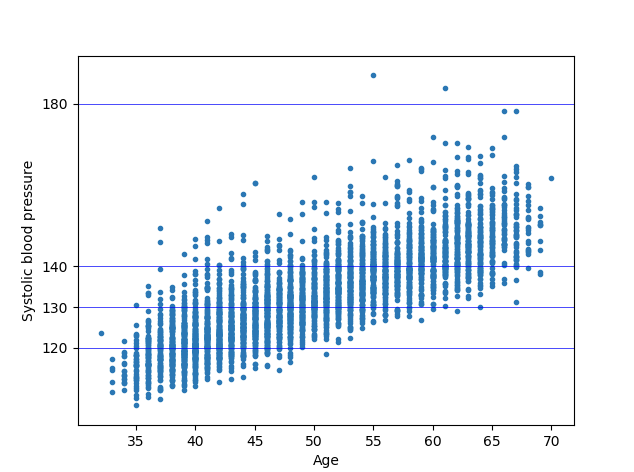
plt.show()We get the below two plots from our regression modals. We can see in the below plots how Age and BMI has an effect on the BMI.