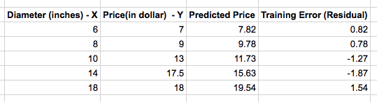
Previously we derived a simple linear regression modal for our Pizza price dataset. We built a modal that predicted a price of $13.68 for a 12 inch pizza. When the same modal is used to predict the price of an 8 inch pizza, we get $9.78 which is around $0.78 more than the known price of $9. This difference between the price predicted by the modal and the observed price in the training set is called the residual or training error. Below table shows the residuals for our training set.
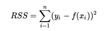
A much better pizza price predictor would be a modal where the sum of training error is as least as possible. We can produce the best pizza-price predictor by minimizing the sum of the residuals. That is, our model fits if the values it predicts for the response variable are close to the observed values for all of the training examples. This measure of model’s fitness is called the residual sum of squares cost function. The residual sum is calculated using the below formula where yi is the observed value and f(xi) is the predicted value.
Lets extend our program from our previous article to calculate the residual sum of squares.
import numpy as np
from sklearn.linear_model import LinearRegression

# Training data
X = [[6], [8], [10], [14],   [18]]
y = [[7], [9], [13], [17.5], [18]]

# Create and fit the model
model = LinearRegression()
model.fit(X, y)

print 'A 12" pizza should cost: $%.2f' % model.predict(12)[0]
#A 12" pizza should cost: $13.68

print np.mean((model.predict(X) - y) ** 2)
#Residual sum of squares: 1.74956896552
We get 1.74 as our cost function or loss function which gives us the measure of error in our modal. The smaller the residual sum of squares, the better your model fits your data; The greater the residual sum of squares, the poorer your model fits your data. A value of zero means your model is a perfect fit.