Abstract
This article presents a method for automatic detection and extraction of number plates from the images of cars. There are usually three steps in an Automatic Number Plate Recognition (ANPR) system. The first one is to binarize the image and separate the background from the foreground. The Foreground contains the numbers of the number plate usually with strong edges. The second step is to identify the number plate in the foreground pixels. The last step is the OCR of the identified number images. Each step has its own set of algorithms.
In this article, I will be focussing on the second step, the extraction of the number plate from the car. I am assuming a good algorithm for thresholding already in place. I will explain good thresholding algorithms in my future posts.
The key idea is to first run a connected component labeling on the thresholded image. Then identify the components with numbers based on the fact that the numbers usually lie in a straight line. The numbers also have similar heights and widths. Even when the number plate is not parallel to the horizontal plane, it still is in a straight line with each other.
Introduction
License plate recognition (LPR), or automatic number plate recognition (ANPR), is the use of video captured images from traffic surveillance cameras for the automatic identification of a vehicle through its license plate. LPR attempts to make the reading automatic by processing sets of images captured by cameras, often setup at fixed locations on roads and at parking lot entrances. ANPR was invented in 1976 at the Police Scientific Development Branch in Britain and since then this had been an actively researched field with many papers published with a goal to make the ANPR systems faster and more accurate in their recognitions.There are seven primary algorithms that the software requires for identifying a license plate as described here in this wikipedia article [4] :
- Plate localization – responsible for finding and isolating the plate on the picture.
- Plate orientation and sizing – compensates for the skew of the plate and adjusts the dimensions to the required size.
- Normalization – adjusts the brightness and contrast of the image.
- Character segmentation – finds the individual characters on the plates.
- Optical character recognition.
- Syntactical/Geometrical analysis – check characters and positions against country-specific rules.
- The averaging of the recognized value over multiple fields/images to produce a more reliable or confident result. Especially since any single image may contain a reflected light flare, be partially obscured, or other temporary effects.
- In this part of the series, I would be focussing on a Plate localization algorithm inspired by multiple previously researched papers [1],[2],[3].
Algorithm
I will threshold the image using Otsu’s method to separate the foreground containing numbers from the background. Then apply the connected component analysis on a car image. The identified labels also contain individual letters on the license plate. One interesting fact about these numbers is that they usually fall in the same line even if the image taken by the camera is skewed. I will use this collinearity property of numbers to isolate them from other connected components in the image.
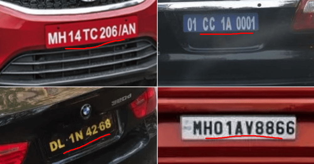
Take a look at the below images of licence plates.
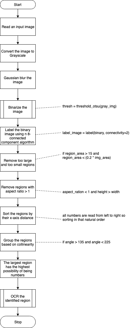
The flow of steps in number plate localisation is in the below diagram:
Implementation:
Let’s go over the steps one by one and understand how it all works out. As usual, the entire implementation notebook can be found here.
Step 1: Read the image and guassian blur and convert it to grayscale
car = imread('http://com.dataturks.a96-i23.open.s3.amazonaws.com/2c9fafb0646e9cf9016473f1a561002a/94c5a151-24b5-493c-a900-017a4353b00c___3e7fd381-0ae5-4421-8a70-279ee0ec1c61_Tata-Tiago-Front-Number-Plates-Design.jpg')
gray_img = rgb2gray(car)
blurred_gray_img = gaussian(gray_img)
plt.figure(figsize=(20,20))
plt.axis("off")
plt.imshow(blurred_gray_img, cmap="gray")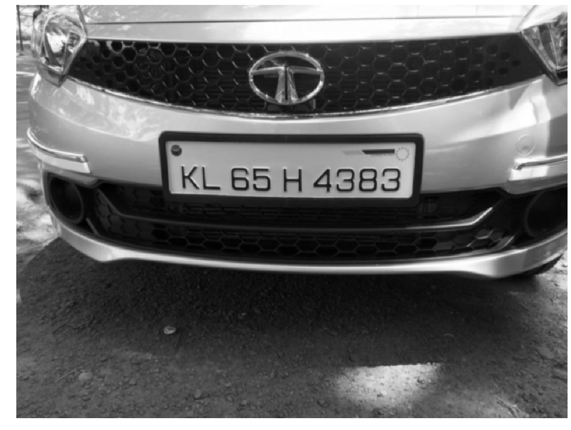
Guassian blur will reduce any potential noise in the image.
Step 2: Binarize the image
I am using the widely used Otsu threshold, though its not the suggested method when it comes to ANPR systems. There are more sophisticated algorithms published only for this step which I will be talking about in my future posts. The image selected by me as a sample works fine with Otsu method.
thresh = threshold_otsu(gray_img)
binary = invert(gray_img > thresh)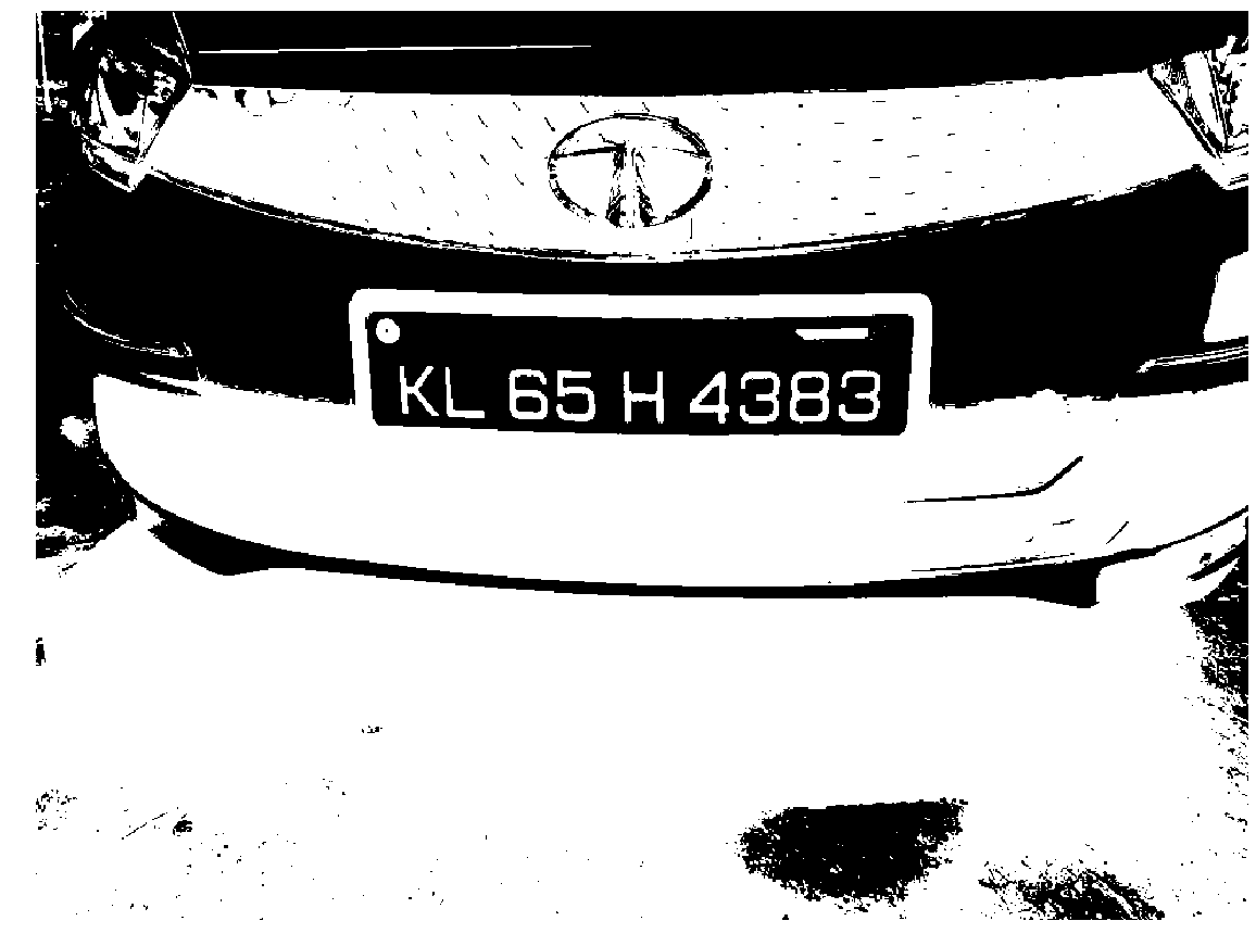
Step 3: Label the binary image using n 8-connected component algorithm
label_image = label(binary, connectivity=2)

fig, ax = plt.subplots(figsize=(10, 6))
ax.axis("off")
ax.imshow(binary, cmap="gray")

for region in regionprops(label_image):
    minr, minc, maxr, maxc = region.bbox
    rect = mpatches.Rectangle((minc, minr), maxc - minc, maxr - minr,
                              fill=False, edgecolor='red', linewidth=2)
    ax.add_patch(rect)

plt.tight_layout()
plt.show()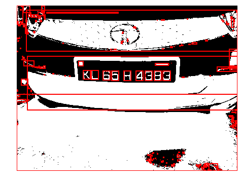
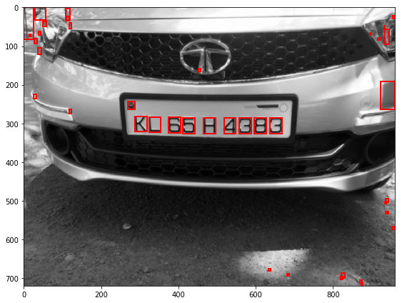
As you can see, there are many connected components found in the image of varied sizes and shapes. I am interested in the ones that make the number plate. As explained in the algorithm section, I would try and remove all the other unwanted components.
Step 4: Remove too large, too small regions and regions whose aspect ratio is greater than 1.
The key idea of this step is to remove the regions which are too big or too small. If the area of the region is less than 15px or greater than 1/5th of the entire image area it probably is not the one which can contain our numbers, ignore them. The standard fonts used in number plates have the width smaller than the height. So, I will remove the components having an aspect ratio less than 1.
fig, ax = plt.subplots(figsize=(10, 6))
ax.imshow(blurred_gray_img, cmap="gray")

# step 1 is to identify regions which probably contains text.
text_like_regions = []
for region in regionprops(label_image):
    minr, minc, maxr, maxc = region.bbox
    w = maxc - minc
    h = maxr - minr

    asr = w/h
    probably_text = False

    region_area = w*h

    # The aspect ratio is constrained to lie between 0.1 and 10 to eliminate
    # highly elongated regions

    # The size of the EB should be
    # greater than 15 pixels but smaller than 1/5th of the image
    # dimension to be considered for further processing

    wid,hei = blurred_gray_img.shape
    img_area = wid*hei

    if region_area > 15 and region_area < (0.2 * img_area) and asr < 1 and h > w:
        #print(w, h, i, region.area, region.bbox)
        probably_text = True

    if probably_text:
        text_like_regions.append(region)

for region in text_like_regions:
    minr, minc, maxr, maxc = region.bbox
    rect = mpatches.Rectangle((minc, minr), maxc - minc, maxr - minr,
                              fill=False, edgecolor='red', linewidth=2)
    ax.add_patch(rect)

plt.tight_layout()
plt.show()
The above image shows regions identified which probably contains text. We can clearly see in the above image that the number plates are collinear. Lets try and isolate them.
Step 5: Sort the regions by how far they are from the Y-axis, group them by their collinearity and pick the largest region.
As mentioned earlier, the numbers are usually collinear. The standard way to check collinearity is to compare the slopes between different points, sort them and group them by slope. But that method will not work for my case here because the corner points of the regions are not perfectly collinear. I would use the angle between the three points to find if the points lie in an almost straight line. I do that by checking if the angle between three points lies between 170 and 190 degrees.
angle = angle_between_three_points(pmin,qmin,rmin)
if angle > 170 and angle < 190:
    cluster.append(r)
Another important way to isolate the components with numbers is to assume that they follow a natural left to right order. So I will sort the components by their distance from the Y-Axis of the image. I will simply sort the identified regions by their column values.
# find the angle between the three points A,B,C
# Angle between line BA and BC
def angle_between_three_points(pointA, pointB, pointC):
    BA = pointA - pointB
    BC = pointC - pointB

    try:
        cosine_angle = np.dot(BA, BC) / (np.linalg.norm(BA) * np.linalg.norm(BC))
        angle = np.arccos(cosine_angle)
    except:
        print("exc")
        raise Exception('invalid cosine')

    return np.degrees(angle)

all_points = np.array(all_points)

all_points = all_points[all_points[:,1].argsort()]
height, width = blurred_gray_img.shape
groups = []
for p in all_points:
    cluster = [p]
    lines_found = False
    for q in all_points:
        pmin = np.array([p[0],p[1]])
        qmin = np.array([q[0],q[1]])
        if p[1] < q[1] and euclidean(pmin,qmin) < 0.1 * width:
            # first check if q is already added, if not add.
            point_already_added = False
            for cpoints in cluster:
                if cpoints[0] == q[0] and cpoints[1] == q[1]:
                    point_already_added = True
                    break;
            if not point_already_added:
                cluster.append(q)

            for r in all_points:
                rmin = np.array([r[0],r[1]])
                last_cluster_point = np.array([cluster[-1][0],cluster[-1][1]])
                if q[1] < r[0] and euclidean(last_cluster_point,rmin) < 0.1 * width:
                    angle = angle_between_three_points(pmin,qmin,rmin)
                    if angle > 170 and angle < 190:
                        lines_found = True
                        cluster.append(r)

    if lines_found:
        groups.append(np.array(cluster))

# plot the longest found line on the image
longest = -1
longest_index = -1
for index, cluster in enumerate(groups):
    if len(cluster) > longest:
        longest_index = index
        longest = len(cluster)

print("coordinates of licence plate\n")
print(groups[longest_index])
Once we have identified the licence plates, we will plot those on the image and the output of it is as shown below.
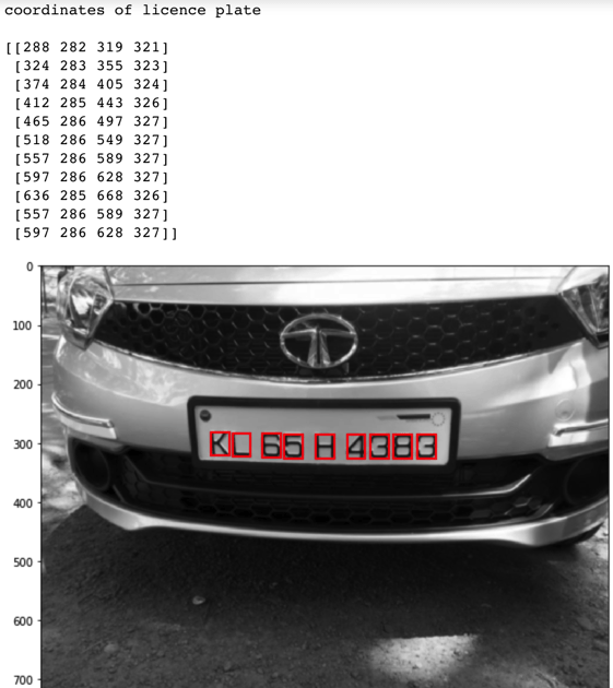
The identified numbers can be further passed into an OCR system to convert into text. I will be covering it in my future posts in this series.
Notes:
The detection of licence plate number depends a lot on the thresholding algorithm, the one I used in this article was the Otsu method which may not be well suited for most binarization techniques. I will be covering a better binarization algorithm in my future posts.
References:
[1] T Kasar, J Kumar and A G Ramakrishnan, “Font and Background Color Independent Text Binarization”
[2] H. Bai and C. Liu, “A hybrid license plate extraction method based on edge statistics and morphology”
[3] Khalid Aboura, “Automatic Thresholding of License Plate Image Data”
[4] Automatic number-plate recognition, Wikipedia
[5] Topological sweeping algorithm of Edelsbrunner and Guibas