Understanding Interquartile Range (IQR) and Outliers

When dealing with a large number of data, It’s a good practice to remove any outliers before further processing unless there is a good reason to keep them. Outliers in simple words are datapoint which are unusually far away from the rest of the dataset.

For the lazy, here is the code to find outliers using IQR in a 1D array.

# pass a 1 D array
def outliers_iqr(ys):
    quartile_1, quartile_3 = np.percentile(ys, [25, 75])
    iqr = quartile_3 - quartile_1
    lower_bound = quartile_1 - (iqr * 1.5)
    upper_bound = quartile_3 + (iqr * 1.5)
    return np.where((ys > upper_bound) | (ys < lower_bound))

# pass a 1 D array
def remove_outliers(array):
  index_outliers = outliers_iqr(array)
  outliers_removed = np.delete(array, index_outliers)
  return outliers_removed

Consider a hypothetical situation where a teacher is given the task of checking if the BMI of her students in the class is within a healthy range. Now after collecting the height and weight data of all her students, it’s important to check for any outlier which may affect the mean calculation. The outlier could also be an experimental error, not removing them may drag the BMI to a value which may not reflect the correct health of her students.

The values removed from the total set is what we call Outliers. There are many ways to remove outliers, one of them is the IQR (Interquartile range) method. IQR gives us the middle 50% of the values from the histogram. The best way to visualize the IQR is through a box plot. Take a look at the below boxplot to get an understanding of IQR.

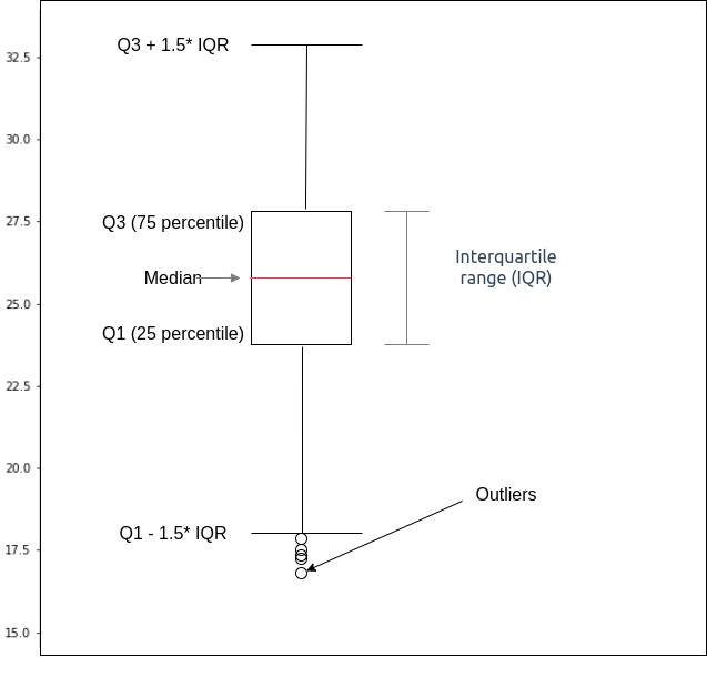
The above diagram makes it clear what data belongs to outlier, the code for it looks like this:

def outliers_iqr(ys):
    # Q1 is 25 percentile, Q3 is 75 percentile
    quartile_1, quartile_3 = np.percentile(ys, [25, 75])
    # IQR is Q3 - Q1
    iqr = quartile_3 - quartile_1
    lower_bound = quartile_1 - (iqr * 1.5)
    upper_bound = quartile_3 + (iqr * 1.5)
    # Anything below the minimum or above the maximum becomes
    # an outlier
    return np.where((ys > upper_bound) | (ys < lower_bound))

As an example, lets look at the same hypothetical use case we discussed previously about BMI. I have a synthetic dataset containing heights and weights of about 30 students. Our goal is to understand how the mean gets affected due to Outliers in the dataset.

Load and Visualize data

import numpy as np
import pandas as pd


data = pd.read_csv('https://muthu.s3-us-west-2.amazonaws.com/dataset/weight-height.csv')

# coverting height from inches to meter
data['Height'] = data['Height'] * 0.0254
# converting weight from pounds to KG
data['Weight'] = data['Weight'] * 0.453592
# BMI = m/h^2
data['BMI'] = data['Weight']/data['Height']**2

print(data)
data.boxplot('BMI', figsize=(10,10))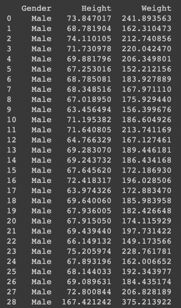

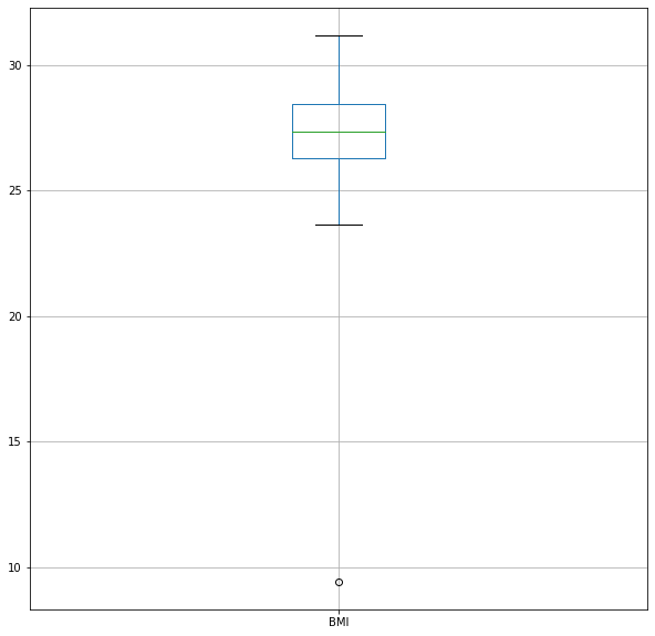
As you can see in the above box plot, there is one record which is way off the rest of the data. This could possibly be an experimental error.

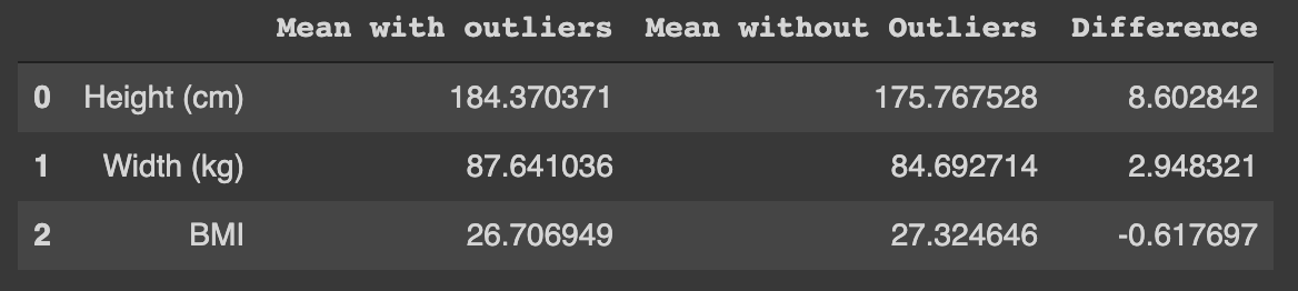
Find the Mean with and without Outliers

# mean on raw data with outliers
h1 = np.mean(data['Height'].to_numpy())
w1 = np.mean(data['Weight'].to_numpy())
b1 = np.mean(data['BMI'].to_numpy())

def outliers_iqr(ys):
    quartile_1, quartile_3 = np.percentile(ys, [25, 75])
    iqr = quartile_3 - quartile_1
    lower_bound = quartile_1 - (iqr * 1.5)
    upper_bound = quartile_3 + (iqr * 1.5)
    return np.where((ys > upper_bound) | (ys < lower_bound))

# pass a 1 D array
def remove_outliers(array):
  index_outliers = outliers_iqr(array)
  outliers_removed = np.delete(array, index_outliers)
  return outliers_removed

# removing outliers and finding the mean
h2 = np.mean(remove_outliers(data['Height'].to_numpy()))
w2 = np.mean(remove_outliers(data['Weight'].to_numpy()))
b2 = np.mean(remove_outliers(data['BMI'].to_numpy()))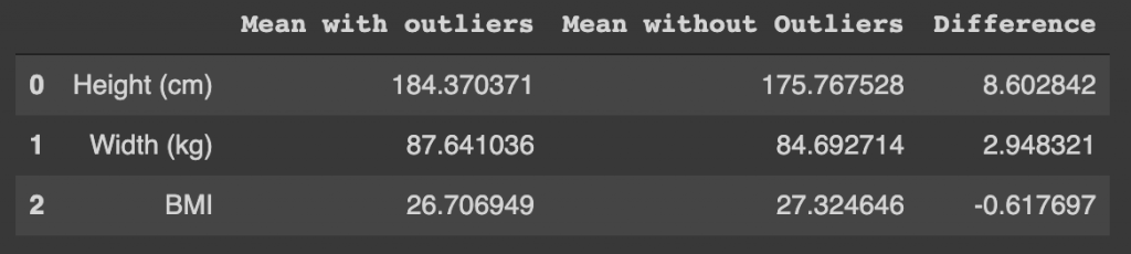

Like I mentioned in the beginning, keeping or removing outliers is a domain knowledge driven decision. You must use your knowledge to decide what values should be discarded from your dataset.