Binomial distribution is used to understand the probability of a particular outcome in repeated independent trials. The probability of a trial is either success or failure. The trials are independent as the outcome or the previous trial had no effect on the next trial, as happens in tossing of coins.
If we flip a coin, it would either be HEADs or TAILs. Normal probability is 0.5 for both p(H) and p(T). In binomial terms we say p(H) is the probability of a HEAD showing up in a trial and 1-p(H) if head doesn’t show up.
If the coin is flipped six times, then getting three heads has the maximum probability, whereas getting a single head or five heads has the least probability. This can be calculated using the below code in python.
from scipy.stats import binom
import matplotlib.pyplot as plt

fig, ax = plt.subplots(1, 1)
x = range(7)
n, p = 6, 0.5
rv = binom(n, p)
ax.vlines(x, 0, rv.pmf(x), colors='k', linestyles='-', lw=1,label='Probablity of Success')
ax.legend(loc='best', frameon=False)
plt.show()
Another example: Suppose a die is tossed 5 times. What is the probability of getting exactly 2 fours?
The probability of any outcome is 1/6=0.167. Our code would look like
from scipy.stats import binom
import matplotlib.pyplot as plt

fig, ax = plt.subplots(1, 1)
x = range(6)
n, p = 5, 0.166
rv = binom(n, p)
ax.vlines(x, 0, rv.pmf(x), colors='k', linestyles='-', lw=1,label='Probablity')
ax.legend(loc='best', frameon=False)
plt.show()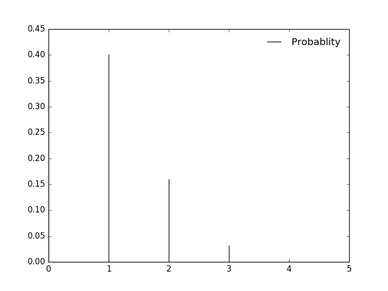
As you can see in the graph above, the probability of second 4 showing up in a throw of a die is 0.161.