Fast nth Fibonacci number algorithm

Definition: The Fibonacci sequence is defined by the equation,

where \(F(0) = 0 \), \(F(1) = 1 \) and \(F(n) = F(n-1) + F(n-2) \text{for } n \geq 2 \). This gives us the sequence 0,1,1,2,3,5,8,13 … called the Fibonacci Sequence.

This post is about how fast we can find the nth number in the Fibonacci series.

Textbook Algorithm

Most textbooks present a simple algorithm for computing the nth Fibonacci number which quickly becomes super slow for larger N. See the implementation below.

# naive fibonacci 
iterations = 0
def fib(n):
    global iterations
    
    if n == 0:
        return 0
    elif n == 1:
        iterations+=1
        return 1
    else:
        iterations+=1
        return fib(n-1) + fib(n-2)

print("sum:", fib(40)) # sum: 102334155
print("total iterations", iterations)  # total iterations 267914295

I have also given the output of the execution in the comment next to the print statement. As you can see, the number of iterations is quite large and if you are running the code in your system you would also notice it takes a few seconds to finish the execution. The running time of this algorithm is exponential which clearly indicates slowness.

Dynamic Programming

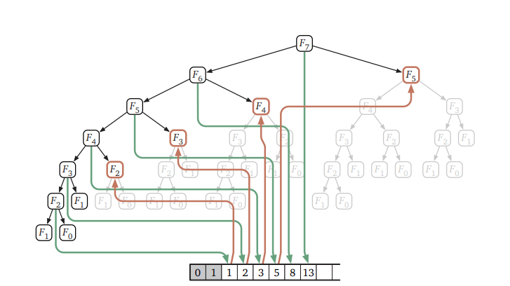
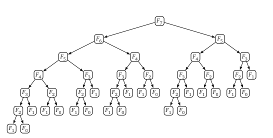
Now to make this algorithm run faster we will have to first look at the recursive calls our algorithm makes to arrive at the nth Fibonacci number.

As you can see In the recursion tree above, most of the values of the right sub tree are calculated more than once, which means, it is computing the same Fibonacci number many times over. So, If we could reduce those calculations we should be able to significantly speed up our algorithm. This is where we use Memoization technique from Dynamic Programming, which is nothing but memorising each new Fibonacci number and  using it in our algorithm to reduce duplicate operations.

Code with memoization

# memoization fibonacci
iterations = 0
def memoize(f):
    memo = {}
    def helper(x):
        if x not in memo:            
            memo[x] = f(x)
        return memo[x]
    return helper

fib = memoize(fib)
print("sum:", fib(40)) # sum: 102334155
print("total iterations", iterations) # total iterations 40

The code only ran 40 iterations! On my machine, the result came instantly. If you trace the calls done after memoization you would notice that most of the right sub tree calculations have been memorised and reused during our computation.

The running time comes down to \(O(n) \) which is evident from the iteration counter.

Another way of memorising the values without using recursion is to keep track of the last two numbers in the fibonacci series. This also runs with the same time complexity of \(O(n) \). Code is given below.

iterations = 0
def fib(n):
    global iterations
    new, old = 1, 0
    for i in range(n):
            new, old = old, new + old
            iterations+=1 #keep track of how many times its run
    return old
print("sum:", fib(40)) #sum:102334155
print("total iterations:", iterations) #total iterations 40

In both the linear and recursive method we calculated the Fibonacci numbers using our knowledge or already calculated Fibonacci numbers. Can we make this algorithm run even more faster? Which takes us to another interesting method using matrices.

Matrix Exponentiation

Take a look at the below matrix:

\begin{align}
\begin{bmatrix}
0 & 1 \\
1 & 1
\end{bmatrix} \begin{bmatrix}
x \\
y
\end{bmatrix} = \begin{bmatrix}
y \\
x + y
\end{bmatrix}
\end{align}

What the above matrix means is, if we multiply a two dimensional vector by \(\begin{bmatrix} 0 & 1 \\  1 & 1 \end{bmatrix} \) we get the same result as we get from our Fibonacci function. So multiplying the matrix n times is the same as iterating the loop n times which implies:

\begin{align}
\begin{bmatrix}
0 & 1 \\
1 & 1
\end{bmatrix}^{n} \begin{bmatrix}
1 \\
0
\end{bmatrix} = \begin{bmatrix}
F_{n-1} \\
F_{n}
\end{bmatrix}
\end{align}

Python code for the matrix method is as below:

import numpy as np
from numpy.linalg import matrix_power

def fibmat(n):
    i = np.array([[0, 1], [1, 1]])
    return np.matmul(matrix_power(i, n), np.array([1, 0]))[1]

print(fibmat(40)) #output : 102334155

Since we are repeatedly squaring and the nth power only takes \(O(logn) \) time. The complexity of our algorithm now reduces to \(O(logn) \) which is a significant improvement over our slow and linear time algorithms.

Double Fibonacci

We can further improve the speed using the below formulas which reduces the number of computations if not the time complexity.

\(F_{2n-1} = F_{n-1}^{2} + F_{n}^{2} \)
\(F_{2n} = F_{n}(2F_{n-1} + F_{n}) \)

The above formula is derived from the Matrix Exponentiation. The code for Double Fibonacci is as given below.

def fib(n):
    if n%2 == 0:#even
        return fib_even(n)
    return fib_odd(n)

def fib_odd(N):
    n = int((N+1)/2)
    Fn = fibmat(n) 
    Fn1 = fibmat(n-1)
    return Fn1**2 + Fn**2

def fib_even(N):
    n = int(N/2)
    Fn = fibmat(n) 
    Fn1 = fibmat(n-1)
    return Fn * (2*Fn1 + Fn)

print(fib(40)) #op: 102334155
print(fib(39)) #op: 63245986

References:

http://jeffe.cs.illinois.edu/teaching/algorithms/book/03-dynprog.pdf
https://docs.scipy.org/doc/numpy/reference/generated/numpy.linalg.matrix_power.html
https://www.nayuki.io/page/fast-fibonacci-algorithms