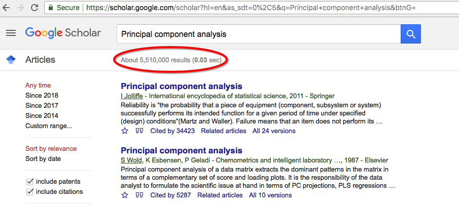
Principal component analysis is a method used to reduce the number of dimensions in a dataset without losing much information. It’s used in many fields such as face recognition and image compression and is a common technique for finding patterns in data and also in the visualization of higher-dimensional data. PCA is all about geometrically projecting the data onto lower dimensions called principal components (PCs). How important PCA is to the machine learning and AI community can only understand by searching the term “Principal Component Analysis” in google scholar. I have added a snapshot of my search result. (28-Aug-2018)
Before diving into the mathematics of PCA, lets compress a sample image using the standard PCA algorithm provided by sklearn. This will give the readers a head start into the power of PCA. For our example I am using the below image.

import matplotlib.image as img
img_data = img.imread('bird.jpg')
print img_data.shape
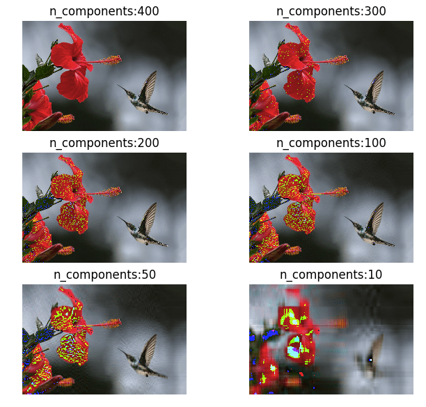
# (467, 700, 3)I have about 700 dimensions in this image as you can see in the output. Let me reduce the dimensions to 400, 300, 200, 100, 50, 10 and restore it back to its original dimensions. Below is the result of my transformations.

As you can see in the above images, we haven’t lost a lot of information until around 50 components. This is why PCA is one of the most important algorithms when it comes to image manipulation and compression.
The full code I used for generating the above analysis is given below:
import matplotlib.image as img
import matplotlib.pyplot as plt
from sklearn.decomposition import PCA
import numpy as np

original_image = img.imread('bird.jpg')
print original_image.shape
print original_image[0]

plt.axis('off')
plt.imshow(original_image)

img_reshaped = np.reshape(original_image, (np.size(original_image, 0),np.size(original_image, 1)*np.size(original_image, 2)))
print img_reshaped.shape

subplot_index = 1
for n_components in [400, 300, 200, 100, 50, 10]:
    plt.subplot(3, 2, subplot_index)
    subplot_index = subplot_index + 1
    ipca = PCA(n_components).fit(img_reshaped)
    transf_img = ipca.transform(img_reshaped)
    #restore the image from the subspace
    image_restored = ipca.inverse_transform(transf_img)
    #reshape the image to the original array size
    image_restored = np.reshape(image_restored, (np.size(original_image, 0),np.size(original_image, 1),np.size(original_image, 2)))
    image_restored = image_restored.astype(np.uint8)
    plt.axis('off')
    plt.title('n_components:' + str(n_components))
    plt.imshow(image_restored)

plt.show()
Now, let’s understand the mathematics behind PCA. First I will attempt to give some elementary background mathematical knowledge required to understand the process of PCA. You can skip the sections with
which you are already familiar with.
Standard Deviation
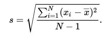
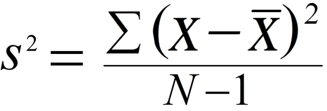
The Standard Deviation (SD) of a data set is a measure of how spread out the data is. A low measure of Standard Deviation indicates that the data is less spread out, whereas a high value means the data is more spread apart from their mean average values. The formula that gives the SD is:
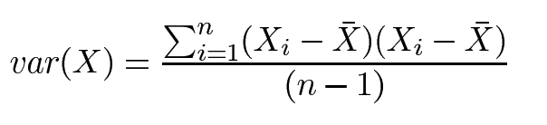
Variance
Variance is another measure of the spread of data in a data set. In fact, it is simply standard deviation squared. The formula is :
Covariance
We use variance and standard deviation only when dealing with 1-dimensional data but for two dimensions we use Covariance. If you think of stock price as a 1-dimensional data moving with time on the x-axis, then we can compare how 2 stocks move together using covariance. Covariance is always measured between 2 dimensions. If you calculate the covariance between one dimension and itself, you get the variance. So, if you had a 3-dimensional data set (x, y, z), then you could measure the covariance between x and y dimensions, the x and z dimensions, and the y and z dimensions. Measuring the covariance between x and x, or y and y, or z and z would give you the variance of the x, y, and z dimensions.
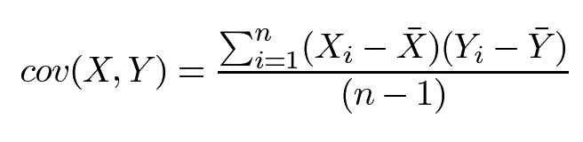
We will use this data to find the correlation as positive or negative. If the value is positive, it indicates that both dimensions are increasing together. If the value is negative, then as one dimension increases, the other decreases.
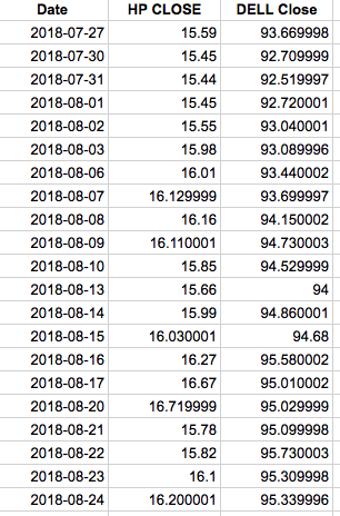
import numpy as np price_HP = [15.59,15.45,15.44,15.45,15.55,15.98,16.01,16.129999,16.16,16.110001,15.85,15.66,15.99,16.030001,16.27,16.67,16.719999,15.78,15.82,16.1,16.200001] price_DELL = [93.669998,92.709999,92.519997,92.720001,93.040001,93.089996,93.440002,93.699997,94.150002,94.730003,94.529999,94,94.860001,94.68,95.580002,95.010002,95.029999,95.099998,95.730003,95.309998,95.339996] mean_HP = np.mean(price_HP) mean_DELL = np.mean(price_DELL) sum = 0 for i in range(len(price_HP)):     sum += (price_HP[i]-mean_HP)*(price_DELL[i]-mean_DELL) covariance = sum/(len(price_HP)-1) print covariance #covariance from numpy library. print np.cov(price_HP,price_DELL)[0][1]

##outputs.
0.23774758583349764
0.23774758583349764
As you can see, the covariance equals ~0.23 which is a positive number, so we can assume the two stocks are moving together.
Covariance Matrix
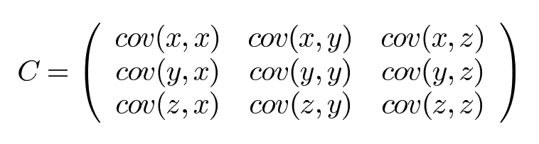
If your dataset has more than 2 dimensions then it can have more than one covariance measurement. For example, if you have a dataset with 3 dimensions x, y and z, then the covariance of this dataset is given by:
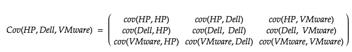
Let’s see how the covariance matrix looks like when we have another stock added to the analysis. This time lets pick VMware price data.
price_VMWARE = [
148.800003,
144.419998,
144.589996,
144.580002,
148.070007,
149.449997,
151.380005,
153.059998,
152.839996,
153.759995,
153.210007,
151.940002,
152.25,
152.039993,
151.929993,
150.880005,
151.619995,
151.679993,
154.279999,
154.770004,
151.369995
]
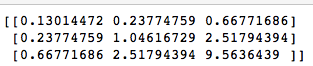
print(np.cov(price_HP,price_DELL,price_VMWARE))The output looks like this:
Eigenvectors and Eigenvalues
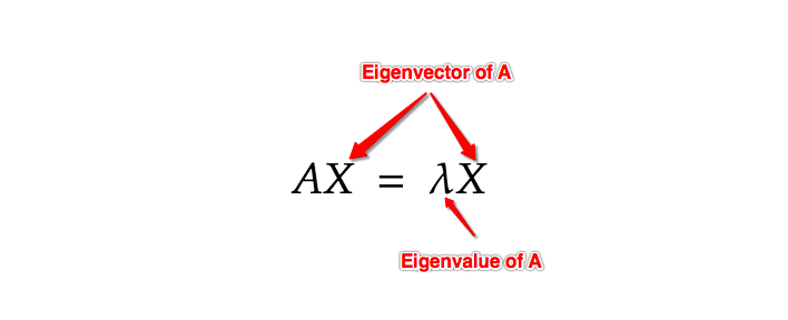
Understanding these two properties is the most important part of understanding PCA. An eigenvector is a vector whose direction remains unchanged when a linear transformation is applied on it. In mathematical terms, an Eigenvector when multiplied to a vector gives a product of the Eigenvector itself with a scalar.
 The best explanation of Eigenvectors and Eigenvalues is given in the below video. I wish I had this video when I learnt about Eigenvectors for the first time.
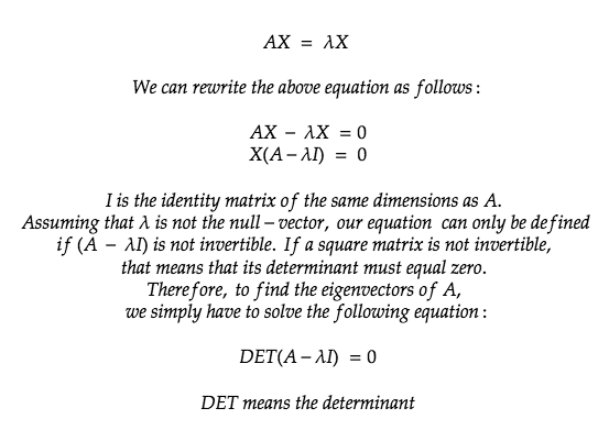
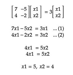
Now, let’s do some maths and find the eigenvector and eigenvalue of a sample vector.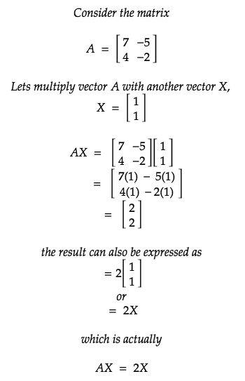
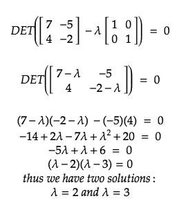
Replacing the value of our vector A in the above formula we get:
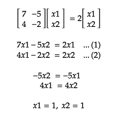
With the found Eigenvalues, let’s try and find the corresponding Eigenvectors which satisfy AX= λX.
For Eigenvector, λ= 2:
For Eigenvector, λ = 3:
-
In short, the Eigenvector is a projection of our dataset onto a subspace and the eigenvector with the highest eigenvalue is the principal component of the data set.
Principal Component Analysis (PCA)
Now that we know the different mathematical concepts involved in PCA let’s put them all together into a sequence of steps to find the components that best describe our higher dimensional data.- Get the dataset.
- Subtract the columns with its mean. For PCA to work, we need to center the data points along the origin by subtracting the points by their mean.
- Find the covariance matrix
- Find the Eigenvectors and Eigenvalues of the covariance matrix
- Choose Eigenvectors (Principal Components) with the highest Eigenvalues and then multiply it with our original data matrix.
We will attempt to project a 2 dimensional to 1 dimension.
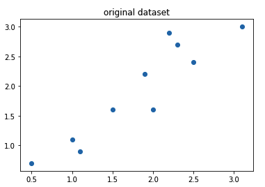
Step 1: Get the dataset
import numpy as np
import matplotlib.pyplot as plt

input = np.array([[2.5 ,2.4],[0.5, 0.7],[2.2 ,2.9],[1.9 ,2.2],[3.1 ,3.0],[2.3 ,2.7],[2 ,1.6],[1 ,1.1],[1.5, 1.6],[1.1 ,0.9]])
print(input)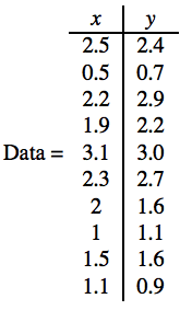
plt.title("original dataset") plt.scatter(input[:,0], input[:,1])
Step 2: Subtract the columns with its mean.
adjusted_input = input - np.mean(input, axis=0)
print("mean adjusted input: ", adjusted_input)
plt.scatter(adjusted_input[:,0], adjusted_input[:,1])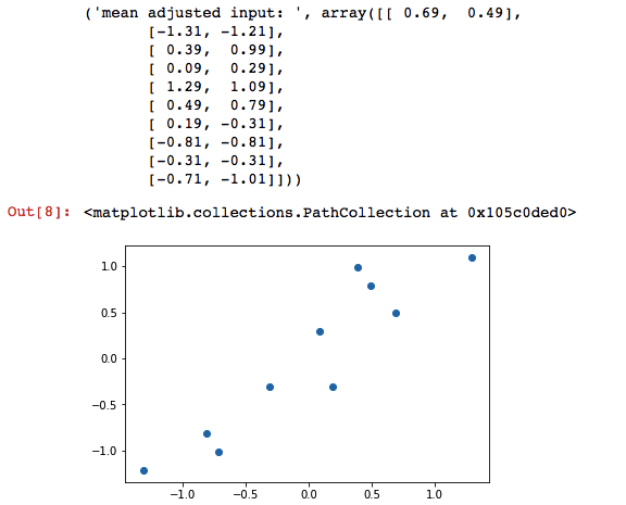
Step 3: Find the covariance matrix
cov = np.cov(adjusted_input[:,0], adjusted_input[:,1])
print(cov) 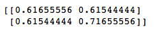
Step 4: Find the Eigenvectors and Eigenvalues of the covariance matrix
from numpy import linalg as LA

w, v = LA.eig(cov)
print("Eigen Value")
print(w)
print("Eigen Vector")
print(v)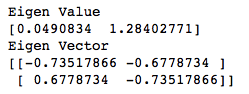
Step 5: Choose Eigenvectors (principal components) with the highest Eigenvalues and then multiply it with our original data matrix.
Of the two eigenvalues 0.0490834 and 1.28402771, 1.28402771 is greater so this becomes our Eigenvalue whose corresponding Eigenvector is the principal component.
#multiply the original data with the eigen vector
eigen_input = np.dot(adjusted_input, np.array(v.T[1]))
print(eigen_input.reshape(10,1))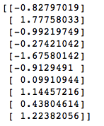
The above array is our lower-dimensional representation of our original dataset in 2D.
The full code is here: PCA from scratch for 2 dimensional dataset.
There is another one that is for 3D data: PCA from scratch for 3 dimensional dataset.ipynb.
PCA’s main weakness is that it gets highly affected by outliers. There are many robust variants of PCA which act to iteratively discard data points that are poorly described by the initial components. Scikit-Learn contains a couple interesting variants on PCA, like RandomizedPCA and SparsePCA, both are present in the sklearn.decomposition submodule of sklearn.
References:
https://stats.stackexchange.com/questions/2691/making-sense-of-principal-component-analysis-eigenvectors-eigenvalues
http://setosa.io/ev/principal-component-analysis/
https://jakevdp.github.io/PythonDataScienceHandbook/05.09-principal-component-analysis.html