Support Vector machines (SVM) can be used for both classification as well as regression tasks but they are mostly used in classification applications. Some of the real world applications include Face detection, Handwriting detection, Document categorisation, SPAM Filtering, image classification and protein remote homology detection. For many researchers, SVM is the first best choice for any classification task because of its efficiency in performing classification on linearly separable as well as non-linear datasets.
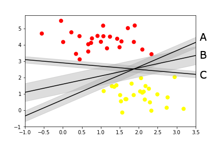
Take a look at the below image, there are multiple lines dividing the two data sets. SVM helps us find the one marked B because its the widest divider between the datasets.
Support Vector machines are based on the concept of finding the best and the widest plane that divides a set of data. The advantage of using SVM over other classification algorithms like K-Means or Naive Bayes is that SVM finds the decision boundary that maximizes the distance from the nearest data points of all the classes. An SVM doesn’t merely find a decision boundary; it finds the most optimal decision boundary. Take a look at the below illustration to understand it better:
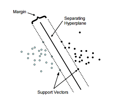
In the above illustration, you can see two set of dots, blue and black divided by a single line called the Hyperplane. The margin is the widest road separating the two sets. As marked in the diagram there are few data points which touch the highest margin line, these are called our support vectors (the reason why this algorithm is called Support Vector Machine).
But not all datasets can be divided by a straight line. Take a look at the below dataset:
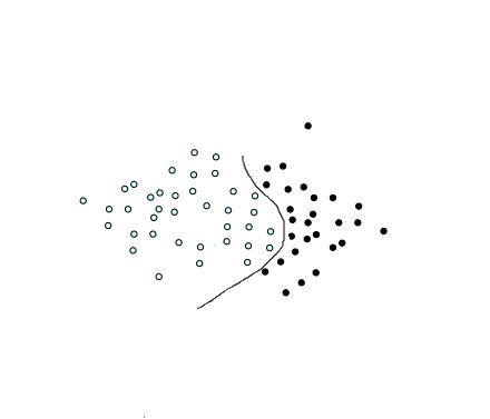
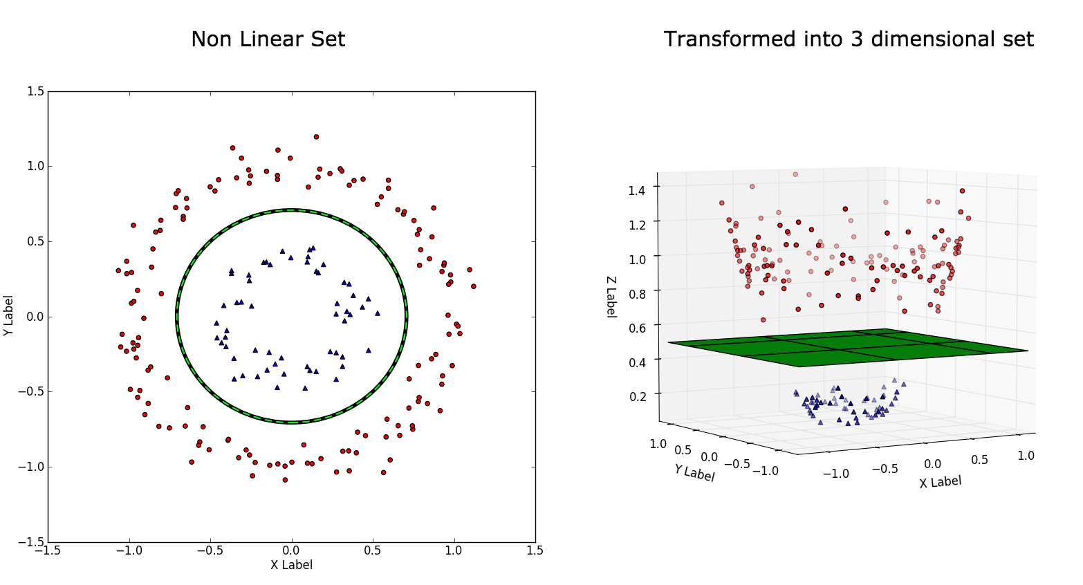
This is the type we call a non-linear dataset which we usually get for our real world applications. We have to transform these into a form which can be linearly separated. We do that by using functions called kernels.
Transforming Linear data using Linear Kernel:
Transforming data using higher order polynomial or gaussian kernel:
Maths behind finding the hyperplane has been nicely explained here, so I will leave the mathematics part and jump right to the implementation.
With the basics in place, first lets try SVM on a random dataset which is linearly separable and understand the various parts of this machine learning algorithm.
# importing scikit learn with make_blobs
from sklearn.datasets.samples_generator import make_blobs
import numpy as np
import pandas as pd
import matplotlib.pyplot as plt

# Y containing two classes
X, y = make_blobs(n_samples=50, centers=2, random_state=0, cluster_std=0.40)
# plotting our dataset
plt.scatter(X[:, 0], X[:, 1], c=Y, s=50, cmap='spring');
df = pd.DataFrame(dict(feature1=X[:,0], feature2=X[:,1], category=y))
Our dataset generated from the above code looks like:
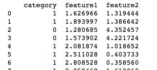
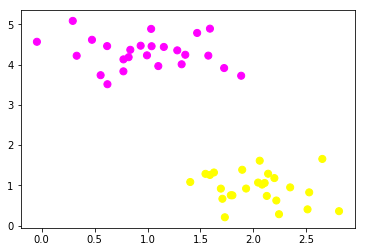
Here “category” is the two groups represented by 0 and 1 for our feature1 and feature2 combination. When plotted we get the below figure, our job using SVM is to find a plane which divides these two datasets.Feeding the above dataset into our SVM :
#split my data set into 80% training and 20% test data
from sklearn.model_selection import train_test_split
X_train, X_test, y_train, y_test = train_test_split(df[['feature1','feature2']], df['category'], test_size = 0.20)

# #the SVM classification of dataset
from sklearn.svm import SVC
svclassifier = SVC(kernel='linear')
svclassifier.fit(X_train, y_train)
y_pred = svclassifier.predict(X_test)
See how simple it is to import SVM algorithm from sklearn and build our prediction modal. Lets evaluate our modal using the classification report:
from sklearn.metrics import classification_report
#evaluating our model for prediction accuracy
print(classification_report(y_test, y_pred))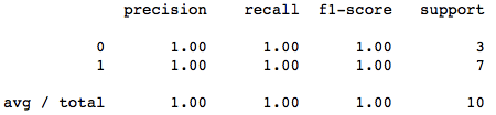
The precision is pretty good. Its 100% accurate for our test data. Now, lets find our hyperplane line and the support vectors and plot them too.
w = svclassifier.coef_[0]
a = -w[0] / w[1]
xx = np.linspace(-5, 5)
yy = a * xx - (svclassifier.intercept_[0]) / w[1]

b = svclassifier.support_vectors_[0]
yy_down = a * xx + (b[1] - a * b[0])
b = svclassifier.support_vectors_[-1]
yy_up = a * xx + (b[1] - a * b[0])

# plot the line, the points, and the nearest vectors to the plane
plt.plot(xx, yy, 'k-')
plt.plot(xx, yy_down, 'k--')
plt.plot(xx, yy_up, 'k--')

plt.scatter(svclassifier.support_vectors_[:, 0], svclassifier.support_vectors_[:, 1],
            s=80, facecolors='none')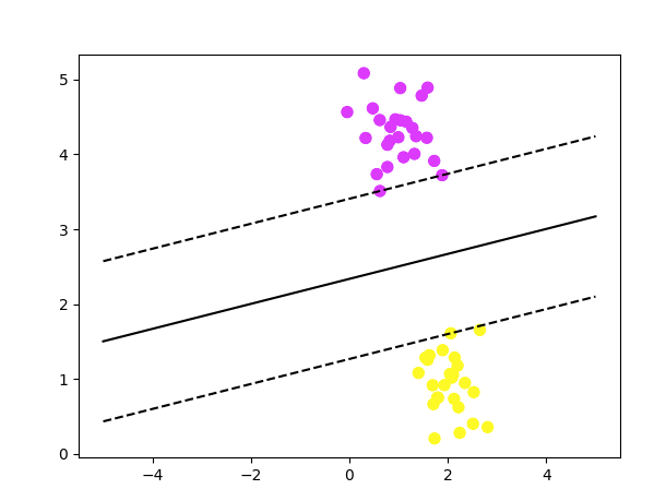
In the above plot, you can see the data set being divided by the most optimal line called the hyperplane and also the support vectors touching the decision boundaries.
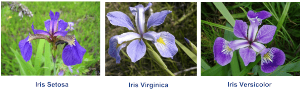
Now, lets try to implement SVM on a real world dataset. For our analysis we will use the famous Iris dataset which consists of 50 samples from each of three species of Iris (Iris setosa, Iris virginica and Iris versicolor). Four features were measured from each sample: the length and the width of the sepals and petals, in centimetres. Based on the combination of these four features we will be building an SVM model to distinguish the species from each other.
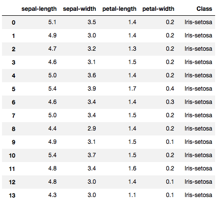
The dataset looks like:
First attempt : Polynomial Kernel – Degree 8
import numpy as np
import matplotlib.pyplot as plt
import pandas as pd
url = "https://archive.ics.uci.edu/ml/machine-learning-databases/iris/iris.data"
#the imported dataset does not have the required column names so lets add it
colnames = ['sepal-length', 'sepal-width', 'petal-length', 'petal-width', 'Class']
irisdata = pd.read_csv(url, names=colnames)
X = irisdata.drop('Class', axis=1) #x contains all the features
y = irisdata['Class'] #contains the categories
#split my data set into 80% training and 20% test data
from sklearn.model_selection import train_test_split
X_train, X_test, y_train, y_test = train_test_split(X, y, test_size = 0.20)
#the SVC algorithm work
from sklearn.svm import SVC
from sklearn.metrics import classification_report, confusion_matrix
svclassifier = SVC(kernel='poly', degree=8)
svclassifier.fit(X_train, y_train)
y_pred = svclassifier.predict(X_test)
#evaluating our model for prediction accuracy
df_cm = confusion_matrix(y_test, y_pred)
print(classification_report(y_test, y_pred))
#seaborn is used for a better looking confusion matrix
import seaborn as sn
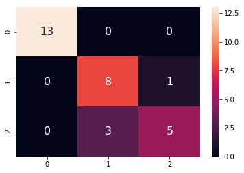
sn.heatmap(df_cm, annot=True,annot_kws={"size": 16})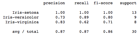
A polynomial kernel is about 87% efficient in classifying the correct flower.
Second Attempt: Gaussian Kernel
There isn’t much to change in our program except changing the parameter kernel to ‘rbf’.
svclassifier = SVC(kernel='rbf')
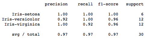
Our classification report now looks like :
Confusion matrix:
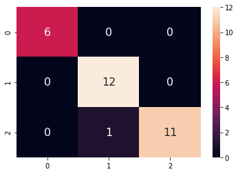
A Gaussian kernel is about 97% accurate in classification.
Amongst the Gaussian kernel and polynomial kernel, we can see that Gaussian kernel prediction was closest to 100% prediction rate while the polynomial kernel was lesser. Therefore the Gaussian kernel performed slightly better. You have to test all the kernels to identify the one which performs best.