Linear Regression using Gradient Descent Algorithm

Gradient descent is an optimization method used to find the minimum value of a function by iteratively updating the parameters of the function. Parameters refer to coefficients in Linear Regression and weights in Neural Networks.

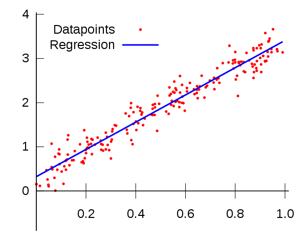
In a linear regression problem, we find a modal that gives an approximate representation of our dataset. In the below image, the red dots denote out dataset, the blue line is what we find using linear regression and the euclidean distance between the red dots and blue line is what we call the cost or the error. You can understand more about linear regression from my previous post.

The equation of line is given by the formula,

where m and b are parameters. Using the gradient descent algorithm we will try to iteratively find the equation of line which produces the least error.  Take a look at the image on how gradient descent finds the line to understand the process visually.

Let (X_i, Y_i) be our dataset, where i is the index and N be the number of data points. The equation of line which can modal our data points is given by,

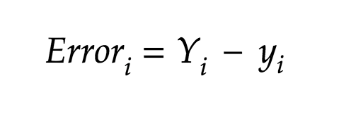
Our modal is not a perfect fit and has error which is the distance between the actual point and the predicted point. The error at each point is given by,

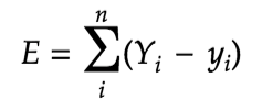
The total error is given by,

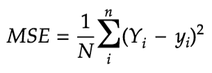
A more formal and widely used method for calculating the total error is Mean Squared Error, which is basically the square of the difference in the actual value and predicted value, we square the difference to avoid negative results. For our analysis we would be using Mean Squared error.

The MSE equation is given by,

which can also be written as,

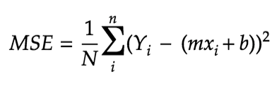
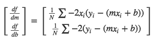
As mentioned earlier, the goal of Gradient Descent is to minimize this equation. So the first step in the process is to find the partial derivatives of the MSE equation wrt. m and b.

Now, to find the values of m and b using gradient descent method, we first start with both m and b with the value of 0. Then we iterate through our datapoints, and at each iteration we adjust the values of m and b using the learning rate and the gradient values. We keep doing it until we have reached our maximum iteration threshold also called epoch or when the cost is at its least. You can see the code below:

learning_rate = 0.01
iterations = 10000

for i in range(iterations):
    
    #find the first derivative of the cost on a and b and minimize it d/da and d/db
    da = 0
    db = 0
    for j in range(len(y)):
        db += -(2/number_of_datapoints) * (y[j] - ((a * X[j]) + b))
        da += -(2/number_of_datapoints) * X[j] * (y[j] - ((a * X[j]) + b))
        
    #adjust a and b
    a = a - (learning_rate * da)
    b = b - (learning_rate * db)
    
    new_cost = np.sum((y - regressed_y)**2)/number_of_datapoints #MSE
    
    #find the convergence point
    if np.sum(costs_reduction[-3:])/costs_reduction[-1:] == 3:
        print "gradient descent convergence point reached at iteration : " + str(i)
        break

You can run the entire working source code here:

Gradient descent implementation of Linear Regression

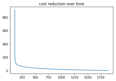
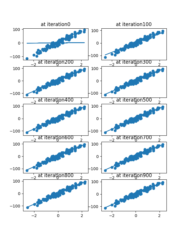
A sample toy dataset implentation gave me the below results. You can see how around 100th iteration the gradient descent started converging towards its minimum.

Below graph shows how the errors came down and became consistent.