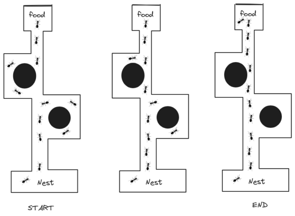
Ant Colony Optimization (ACO) is a metaheuristic optimization algorithm inspired by the foraging behavior of ants. Ants are social insects that communicate with each other using pheromones, which are chemicals that they leave on trails. When an ant finds a good source of food, it will lay down a trail of pheromones on the way back to the nest. Other ants will follow this trail, and the more ants that follow a trail, the stronger the pheromone trail will become. This will eventually lead to a situation where most of the ants are following the shortest path to the food source.
ACO algorithms work by simulating this behavior of ants. They do this by creating a population of artificial ants that are placed in a virtual environment. The ants are then allowed to explore the environment and leave pheromones on the paths that they take. The pheromone trails will evaporate over time, also known as decaying, so the ants will eventually be more likely to follow paths that have been recently used.
Explanation of Ant Colony Optimization
Let’s understand ACO by applying it to the Traveling Salesman Problem. Here’s a high-level overview.
- Initialization: ACO begins by randomly placing a number of ants on different cities.
- Construction of solutions: Each ant constructs a solution by iteratively selecting the next city to visit based on a combination of pheromone trails and heuristic information (e.g., distance between cities).
- Local pheromone deposition: After each ant selects a city, it deposits pheromone on the visited edge to reinforce the attractiveness of that edge.
- Global pheromone update: After all ants have completed their tours, the pheromone trails are updated. The amount of pheromone deposited on each edge depends on the quality of the solution found by the ant.
- Iteration: Steps 2-4 are repeated for a certain number of iterations or until a stopping criterion is met.
- Solution selection: At the end of the iterations, the best solution found by the ants is selected as the final solution to the TSP.
Pheromone Matrix
The pheromone matrix is a two-dimensional matrix that represents the pheromone levels on the edges of the graph in the ACO algorithm. The TSP specifically uses the pheromone matrix to store pheromone levels on each edge connecting two cities. The pheromone levels are updated by the ants during the construction of their paths. The more ants that traverse a particular edge, the higher the pheromone level on that edge becomes.
The pheromone matrix serves as a form of communication between the ants, allowing them to share information indirectly about the quality of different paths. Ants tend to follow paths with higher pheromone levels, as they are considered more attractive. Over time, the pheromone levels on shorter paths tend to increase due to the effect of many ants choosing those paths.
The following pheromone matrices represent the pheromone levels across iterations, from the beginning to the end of the ACO algorithm. As the iterations progress, the pheromone levels of the less optimal paths gradually decrease within the matrices, while those of the best solutions become stronger.
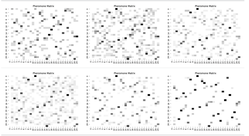
Updating and decaying pheromone levels in the matrix enables the exploration of different paths by the ACO algorithm, eventually leading it to converge towards an optimal or near-optimal solution to the TSP.
Decay Rate
The decay rate determines how quickly the pheromone levels on the edges of the graph decrease over time. Decaying the pheromone levels helps the ACO algorithm avoid getting trapped in suboptimal solutions. This allows it to explore new paths and maintain a balance between exploration and exploitation.
A higher decay rate will cause the pheromone levels to decrease more rapidly, leading to more exploration and less exploitation. Conversely, a lower decay rate will result in slower decay, allowing the algorithm to exploit good paths for a longer time.
A commonly used default value for the decay rate is 0.5. This value allows for a moderate decay of pheromone levels, striking a balance between exploration and exploitation. It is a good starting point for many problems, but it may not always produce the best results. It’s important to note that the decay rate is a parameter that can be adjusted by the user to influence the behavior of the ACO algorithm. Different problems and specific problems may require different decay rates to achieve optimal performance.
Implementation
Below is a simple Python program for solving the Traveling Salesman Problem (TSP) using ACO. This example assumes a complete graph (every pair of cities is connected) and uses the distance between cities as the heuristic information.
import numpy as np


class AntColony:
    def __init__(self, distance_matrix, num_ants,
                    num_iterations, decay_rate, alpha=1.0, beta=2.0):
        self.distance_matrix = distance_matrix
        self.num_ants = num_ants
        self.num_iterations = num_iterations
        self.decay_rate = decay_rate
        self.alpha = alpha
        self.beta = beta
        self.num_cities = distance_matrix.shape[0]
        self.pheromone_matrix = np.ones(
                            (self.num_cities, self.num_cities))
        self.best_path = None
        self.best_path_length = float('inf')

    def run(self):
        for iteration in range(self.num_iterations):
            paths = self.construct_paths()
            self.update_pheromone(paths)
            best_path_index = np.argmin(
                [self.path_length(path) for path in paths])
            if (self.path_length(paths[best_path_index])
                    < self.best_path_length):
                self.best_path = paths[best_path_index]
                self.best_path_length = self.path_length(
                    paths[best_path_index])

            self.pheromone_matrix *= self.decay_rate
            print(self.best_path_length)

    def construct_paths(self):
        paths = []
        for ant in range(self.num_ants):
            visited = [0]  # Start from city 0
            cities_to_visit = set(range(1, self.num_cities))
            while cities_to_visit:
                next_city = self.select_next_city(visited[-1],
                                                cities_to_visit)
                visited.append(next_city)
                cities_to_visit.remove(next_city)
            paths.append(visited)
        return paths

    def select_next_city(self, current_city, cities_to_visit):
        pheromone_values = [
            self.pheromone_matrix[current_city][next_city] ** self.alpha
                            for next_city in cities_to_visit]
        heuristic_values = [
            1.0 / self.distance_matrix[current_city][next_city] ** self.beta
                            for next_city in cities_to_visit]
        probabilities = np.array(pheromone_values) * np.array(
                                                        heuristic_values)
        probabilities /= np.sum(probabilities)
        return list(cities_to_visit)[
                            np.random.choice(range(len(cities_to_visit)),
                                                p=probabilities)]

    def update_pheromone(self, paths):
        for path in paths:
            path_length = self.path_length(path)
            for i in range(len(path) - 1):
                current_city, next_city = path[i], path[i + 1]
                self.pheromone_matrix[current_city][next_city] += 1.0 / path_length

    def path_length(self, path):
        length = 0
        for i in range(len(path) - 1):
            current_city, next_city = path[i], path[i + 1]
            length += self.distance_matrix[current_city][next_city]
        return length


def euclidean_distance(c1, c2):
    # This method calculates the Euclidean distance between two points.
    return np.linalg.norm(c1 - c2)


def adjacency_matrix(coordinate):
    # This method calculates the adjacency matrix for a
    # given set of coordinates.
    # The adjacency matrix represents the distances between
    # each pair of coordinates.
    # It takes a list of coordinates as input and returns a
    # numpy array representing the adjacency matrix.
    matrix = np.zeros((len(coordinate), len(coordinate)))
    for i in range(len(coordinate)):
        for j in range(i + 1, len(coordinate)):
            p = euclidean_distance(coordinate[i], coordinate[j])
            matrix[i][j] = p
            matrix[j][i] = p
    return matrix


# Latitude longitude of cities.
berlin52 = np.array([[3.3333, 36.6667],
                     [6.1333, 35.75],
                     [2.8, 32.2],
                     [1.5, 34.5333],
                     [8.9, 33.4833],
                     [5.8333, 29.25],
                     [6.8333, 37.6667],
                     [7.8, 35.43],
                     [2, 31.5],
                     [6.8333, 31.1667],
                     [5, 30],
                     [3.1167, 37.3333],
                     [10.3333, 40.3333],
                     [2.5, 32.9667],
                     [9.3333, 34.8333],
                     [6.8333, 39.2],
                     [5, 39.6167],
                     [7, 39],
                     [9.9667, 39.6333],
                     [6.3333, 30],
                     [7.9667, 32.4833],
                     [4.1667, 34.25],
                     [7, 31.5],
                     [10.3333, 36],
                     [5.75, 34.9833],
                     [2.1667, 37.6],
                     [6, 34.5],
                     [5.0333, 32.8333],
                     [5.0833, 39.0333],
                     [5.04, 39.43]])

distance_matrix = adjacency_matrix(berlin52)

# Set the parameters
num_ants = 10
num_iterations = 100
decay_rate = 0.5

# Create the AntColony instance and run the algorithm
aco = AntColony(distance_matrix, num_ants, num_iterations, decay_rate)
aco.run()

# Get the best path found
best_path = aco.best_path
best_path_length = aco.best_path_length

# Print the result
print("Best Path:", best_path)
print("Best Path Length:", best_path_length)
In this code, we define a AntColony class that encapsulates the ACO algorithm. The distance_matrix represents the distances between cities. The algorithm is run for a specified number of ants and iterations, with a decay rate to update the pheromone levels. The run() method runs the algorithm, while the construct_paths() method constructs the paths for each ant. The select_next_city() method selects the next city to visit based on the pheromone levels and heuristic values. The update_pheromone() method updates the pheromone levels based on the paths found by the ants. The path_length() method calculates the length of a given path.
To use the code, you can replace the distance_matrix with your own distance values and adjust the parameters num_ants, num_iterations, and decay_rate as desired. The best path and its length will be printed at the end.
Visualization
Let’s visualize the ACO algorithm with the dataset we used for visuaizing Tabu search in our previous chapters.
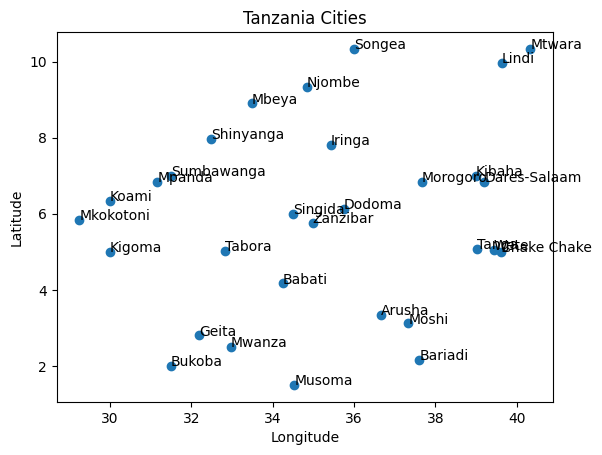
The program runs for 100 iterations and after each iteration checks if the discovered path is better than the previously saved best path length. Below is a visualization of the best paths discovered over 100 iterations.
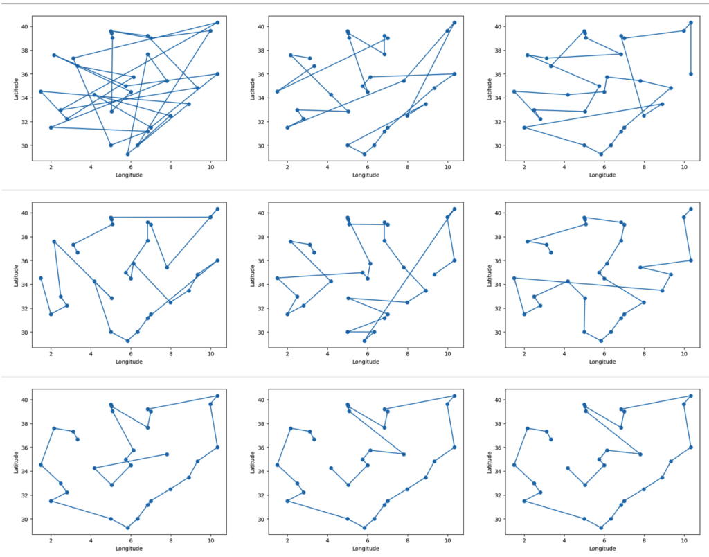
Over the 100 iterations, the total distance gradually improves and converges to the best path. The graph below illustrates the convergence over the iterations.
Advantages
- Efficient exploration and exploitation: ACO balances the exploration of new solutions in the search space with the exploitation of promising solutions already found. This allows ACO to avoid getting stuck in local optima and find high-quality solutions efficiently.
- Adaptability and robustness: ACO algorithms are highly adaptable to different problem domains and can handle complex problems with large search spaces. They are also robust to changes in the problem environment and noise in the data.
Limitations
- Parameter tuning: ACO algorithms require careful tuning of several parameters to achieve optimal performance. This can be a time-consuming and challenging process, especially for complex problems.
- Premature convergence: In some cases, ACO algorithms can prematurely converge to a suboptimal solution. This can occur if the pheromone trails become too concentrated around a particular solution, leading the ants to explore a limited area of the search space.
Additional points to consider:
- ACO algorithms may require more computational resources compared to other metaheuristics.
- The performance of ACO can vary depending on the specific problem and the chosen algorithm variant.
Despite these limitations, ACO remains a powerful and versatile optimization algorithm with numerous applications across various domains. Its advantages of efficient exploration and exploitation, adaptability, and robustness make it a valuable tool for solving complex problems in finance, logistics, engineering, and many other areas.
Applications
Logistics and Routing:
- Vehicle Routing Problem (VRP): ACO algorithms are widely used to optimize delivery routes for vehicles, minimizing travel distances and fuel consumption.
- Traffic Light Control Optimization: ACO can be applied to dynamically adjust traffic light timings based on real-time traffic data, improving traffic flow and reducing congestion.
- Scheduling and Planning: ACO algorithms can be used to optimize task scheduling, resource allocation, and other planning problems in various industries.
Finance and Economics:
- Portfolio Optimization: ACO can help investors create diversified portfolios with optimal risk-reward ratios.
- Credit Risk Assessment: ACO can be used to analyze financial data and assess the creditworthiness of borrowers.
- Market Prediction: ACO algorithms can analyze market trends and predict future prices of various assets.
This algorithm and many more are explained in my “Essential Search Algorithms” book.